AMR’s contribution is a reproducible reconciliation of the paper’s selected printed endpoints, published percentage summaries and statistical definitions. The comparison covers two injection cases, three first-year wastewater cases and two forms of normalized water input. It preserves the original historical periods. It does not estimate a current US average, a freshwater share or a lifetime wastewater volume.
A central distinction runs through the evidence: the source groups injection records by spud year, while its production analysis groups wells by first-production year and month since production began. First-year flowback and produced water is constructed from monthly medians over the first 12 production months. Those regional summaries should not be treated as a traced water balance for the same individual well. Kondash and colleagues, Materials and Methods.
Key Takeaways
- The Permian injection comparison is historical. AMR calculates a 767.3469% change from the printed 2011 and 2016 endpoints; the paper summarizes this case at about 770%.
- Marcellus has a different reported input change. Its printed median endpoints, 23,400 and 27,950 m³ per well, yield an AMR calculation of 19.4444% for 2011 to 2016.
- The Eagle Ford gas first-year wastewater endpoints are 1,340 and 20,700 m³ per well. They describe 2011 and 2015 first-production cohorts and yield 1444.7761% by printed-endpoint arithmetic.
- Eagle Ford oil also ends in 2015 in this comparison. Its first-year endpoints are 2,400 and 16,900 m³ per well.
- Niobrara’s printed first-year endpoints are 1,800 and 2,300 m³ per well, for 2011 and 2016 cohorts.
- Per-well, per-lateral-length and per-energy inputs answer different questions. Their denominators remain explicit in the tables.
- Flowback and produced water includes formation water. It is not simply the same injected water returning to the surface.
- AMR calculations reproduce printed values. They do not reconstruct original well records, uncertainty intervals or unobserved current conditions.
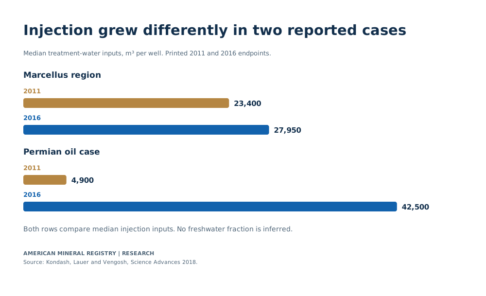
How much did injected water per well change in the reported cases?
The printed Marcellus injection endpoints imply a 19.4444% increase, while the Permian endpoints imply a 767.3469% increase between 2011 and 2016. AMR calculates both from the source’s reported median volumes, retaining their regional case boundaries. The paper summarizes the increases at approximately 20% and 770%. Kondash and colleagues, Results, injection discussion and Fig. 2.

View chart data
Median treatment-water inputs, m3 per well. Printed 2011 and 2016 endpoints.
| Source case | 2011 median injection (m3 per well) | 2016 median injection (m3 per well) |
|---|---|---|
| Marcellus region | 23400 | 27950 |
| Permian oil case | 4900 | 42500 |
Historical selected cases from Kondash et al. 2018, not current US averages.
Source-period and statistical definitions apply; AMR endpoint arithmetic does not reconstruct original uncertainty.
Kondash, Lauer and Vengosh, 2018, Results and Fig. 2 Kondash, Lauer and Vengosh 2018; Results paragraph 1; Fig.2
| Source case | Start year | End year | Start median injection (m3 per well) | End median injection (m3 per well) | AMR absolute change (m3 per well) | AMR change from printed endpoints (%) | Source scope |
|---|---|---|---|---|---|---|---|
| Marcellus region | 2011 | 2016 | 23400 | 27950 | 4550 | 19.4444 | Pennsylvania and West Virginia regional case; source Results injection discussion |
| Permian oil case | 2011 | 2016 | 4900 | 42500 | 37600 | 767.3469 | Texas and New Mexico regional endpoint case; oil-case identification in Results |
The source describes Marcellus in Pennsylvania and West Virginia and the Permian in Texas and New Mexico. Its later discussion identifies the approximately 770% water-use increase with oil-producing wells in the Permian. AMR retains that case qualification rather than presenting the endpoint as the requirement of every Permian well or a universal quantity for hydraulic fracturing.
The arithmetic has a straightforward denominator. For the Permian case, subtracting 4,900 from 42,500 gives an additional 37,600 m³ per well in the printed median comparison. Dividing that increment by the 2011 endpoint produces the percentage change. For Marcellus, the corresponding increment is 4,550 m³ per well. The starting quantities differ, so an increase measured in cubic metres and an increase measured in percent communicate different aspects of the comparison.
A per-well median is also a specific statistic. The source’s injection analysis assigns FracFocus water-use records spatially to regions, then calculates median water use by spud year. It is not a basin’s total annual water volume. Estimating a regional total would require compatible well or treatment counts and a method appropriate to the distribution of quantities. Multiplying a reported median by an unrelated count would introduce a new estimate with assumptions that these tables do not establish. Kondash and colleagues, Statistical methods.
The unit does not identify the source of the water. A treatment-water volume alone cannot be relabeled freshwater withdrawal, groundwater pumping or net freshwater consumption. Those descriptions require evidence about the water source and the relevant accounting boundary. AMR preserves the measured input label and makes no estimate of the freshwater fraction in these historical cases.
These endpoints can support a clear historical statement: the reported median water input changed substantially, and differently, in the named regional comparisons. They cannot establish what a new well requires today or how all basins changed. That narrower use remains valuable because the reader can identify the geography, statistic, date and calculation without reconstructing the paper’s entire analytical system.
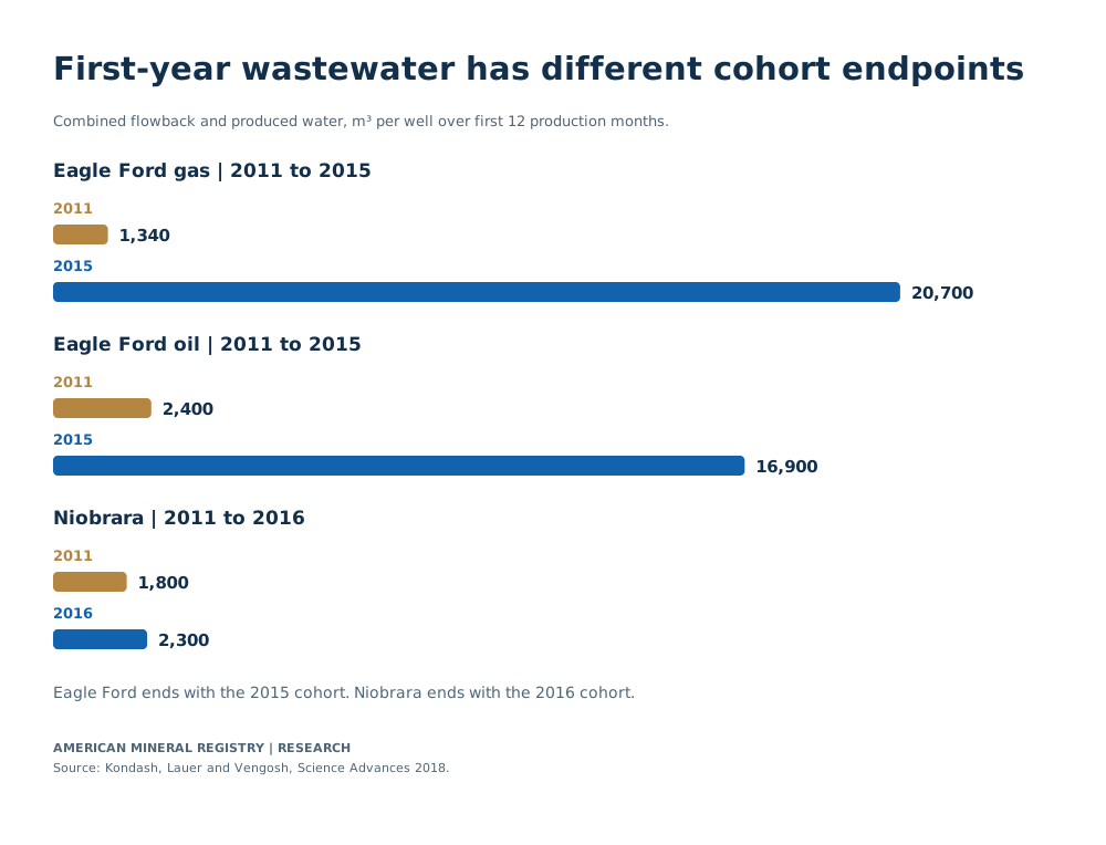
How much first-year flowback and produced water did the study report?
The printed first-year wastewater endpoints increase from 1,340 to 20,700 m³ per well in Eagle Ford gas and from 2,400 to 16,900 m³ in Eagle Ford oil, comparing 2011 with 2015 cohorts. Niobrara’s printed comparison runs from 1,800 m³ in 2011 to 2,300 m³ in 2016. These are combined flowback and produced-water quantities over the first 12 production months. Kondash and colleagues, Results, FP water discussion and Fig. 3.

View chart data
Combined flowback and produced water, m3 per well over first 12 production months.
| Source case | Start cohort | End cohort | Start FP (m3 per well) | End FP (m3 per well) |
|---|---|---|---|---|
| Eagle Ford gas | 2011 | 2015 | 1340 | 20700 |
| Eagle Ford oil | 2011 | 2015 | 2400 | 16900 |
| Niobrara | 2011 | 2016 | 1800 | 2300 |
Historical selected cases from Kondash et al. 2018, not current US averages.
Source-period and statistical definitions apply; AMR endpoint arithmetic does not reconstruct original uncertainty.
Kondash, Lauer and Vengosh, 2018, Results and Fig. 3 Kondash, Lauer and Vengosh 2018; Results paragraph 2; Fig.3
| Source case | Start first-production cohort | End first-production cohort | Start year-1 FP water (m3 per well) | End year-1 FP water (m3 per well) | AMR absolute change (m3 per well) | AMR change from printed endpoints (%) | Observation boundary |
|---|---|---|---|---|---|---|---|
| Eagle Ford gas | 2011 | 2015 | 1340 | 20700 | 19360 | 1444.7761 | Combined flowback and produced water; first 12 months, not lifetime |
| Eagle Ford oil | 2011 | 2015 | 2400 | 16900 | 14500 | 604.1667 | Combined flowback and produced water; first 12 months, not lifetime |
| Niobrara | 2011 | 2016 | 1800 | 2300 | 500 | 27.7778 | Combined flowback and produced water; first 12 months, not lifetime |
The distinction between calendar year and well age matters here. “First year” means the first 12 months after production begins, aligned by production month for the source’s analysis. It does not mean all wastewater produced by all wells operating in a particular calendar year. Older wells can continue to produce water outside this observation window, so the early quantity is not a lifetime total.
The source’s statistical construction is equally specific. It calculates a median among reporting wells for each month since first production and adds the first 12 monthly medians to form its year-one estimate. That procedure differs from calculating each individual well’s annual total and then taking the median of those totals. The statistics cannot be assumed identical, even though both may be described informally as a typical first-year well. Kondash and colleagues, Statistical methods.
The ending-year difference follows the paper’s coverage decisions. Its statistical methods remove Eagle Ford gas and oil production data for 2016 under a low reporting-coverage screen. The printed FP endpoint cases therefore stop in 2015. A chart using the abstract’s overall 2011 to 2016 study window as the label for every individual row would misdate those endpoints. Niobrara’s printed comparison does reach 2016.
AMR calculates the Eagle Ford gas increment as 19,360 m³ per well, compared with 14,500 m³ for the oil case and 500 m³ for Niobrara. The gas case starts from a lower printed baseline than the oil case, which contributes to its larger percentage increase. Those differences should be described with the row’s basin, production case and cohort window rather than generalized to all shale development.
Finally, FP water is a mixture. The paper describes returned injected treatment water combined with saline formation water entering the well. A larger FP volume can represent more than a larger return of the originally injected fluid. The source’s volume comparison does not separate the origin of every unit of water. That distinction becomes decisive when moving from wastewater management to claims about injection recovery or freshwater consumption.
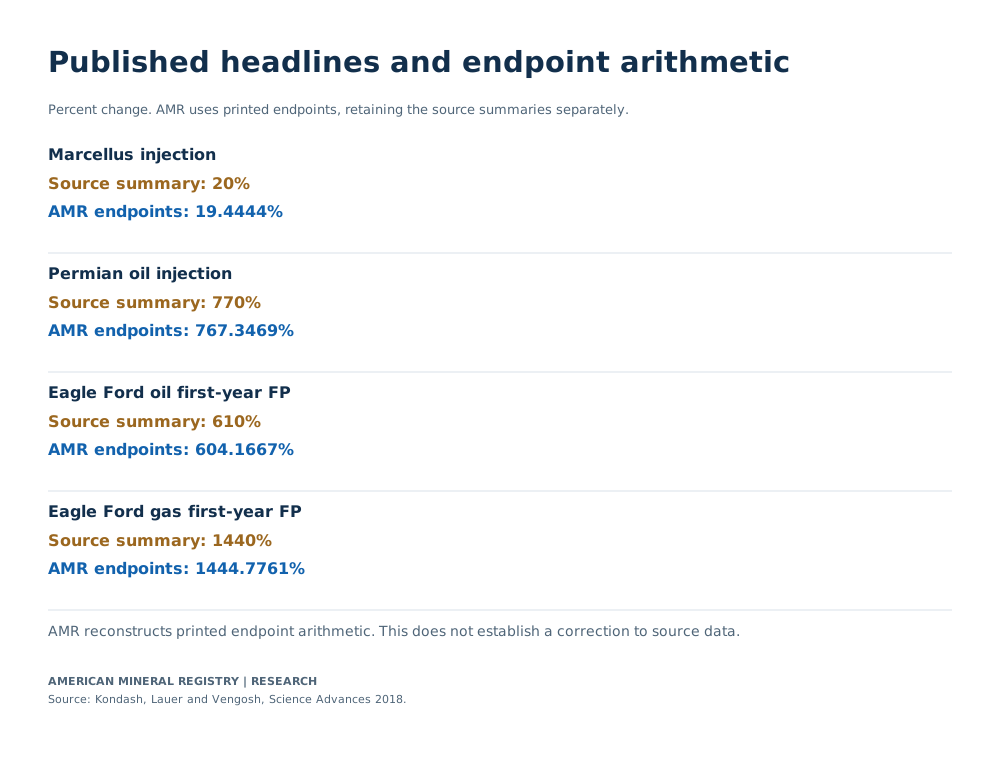
What do the 770% and 1440% headlines actually reproduce?
The source’s approximately 770% injection headline and approximately 1440% first-year wastewater headline describe different cases and endpoint windows. AMR’s arithmetic from the printed endpoints gives 767.3469% for the Permian injection case and 1444.7761% for Eagle Ford gas FP water through the 2015 cohort. Published summary percentages and AMR recomputations remain separate. Kondash and colleagues, Abstract and Results.

View chart data
Percent change. AMR uses printed endpoints, retaining the source summaries separately.
| Comparison | Published source increase (%) | AMR printed-endpoint increase (%) |
|---|---|---|
| Marcellus injection | 20 | 19.4444 |
| Permian oil injection | 770 | 767.3469 |
| Eagle Ford oil first-year FP | 610 | 604.1667 |
| Eagle Ford gas first-year FP | 1440 | 1444.7761 |
Historical selected cases from Kondash et al. 2018, not current US averages.
Source-period and statistical definitions apply; AMR endpoint arithmetic does not reconstruct original uncertainty.
Kondash, Lauer and Vengosh, 2018, Results, reported percentages and accompanying endpoint sentences Kondash, Lauer and Vengosh 2018; Results paragraphs 1 and 2
| Comparison | Start year | End year | Published source increase (%) | AMR recomputation from printed endpoints (%) | AMR minus published (percentage points) | Interpretation |
|---|---|---|---|---|---|---|
| Marcellus injection | 2011 | 2016 | 20 | 19.4444 | -0.5556 | Displayed endpoint arithmetic; retains source summary separately |
| Permian oil injection | 2011 | 2016 | 770 | 767.3469 | -2.6531 | Source up-to injection headline belongs to this historical case |
| Eagle Ford oil first-year FP | 2011 | 2015 | 610 | 604.1667 | -5.8333 | First-year wastewater cohort endpoint comparison stops in 2015 |
| Eagle Ford gas first-year FP | 2011 | 2015 | 1440 | 1444.7761 | 4.7761 | Source up-to FP headline; recomputation is not an original-data correction |
Percent increase uses the earlier quantity as its denominator: (later / earlier − 1) × 100. A large percentage may therefore reflect both a later increase and a low starting value. It is different from the endpoint multiple itself. In a sentence using the paper’s summary, retain “increased by approximately 770%”; do not turn that into “became 770 times larger”.
The printed volumes are already rounded source values. Recomputing them to four decimal places produces a transparent result from those displayed inputs, without recovering the unrounded source observations. The published percentage need not be numerically identical to that recomputation. The table makes the difference inspectable while keeping the original authors’ characterization visible.
This treatment is especially useful for Eagle Ford oil. Its published summary is 610%, while 16,900 / 2,400 yields a 604.1667% increase from the printed endpoints. AMR reports the calculation and its premise rather than silently replacing the source’s figure or claiming to have resolved its original-data basis. The extra decimal places belong to the calculation, rather than an uncertainty claim about the physical water volume.
A second source of confusion is the phrase “up to”. The cited maxima describe particular cases in the historical study. They are not average increases across all US wells, a minimum applying to every basin or a current annual growth rate. Nor can the injection maximum and wastewater maximum be combined into a single well’s water balance: their regional cases, cohort clocks and ending years differ.
For a broad historical quotation, the paper’s approximate headline can be used with its case and period attached. For an audit of displayed values, cite the AMR endpoint calculation and its matching CSV. For a new estimate of actual conditions, neither number substitutes for the required current observations. Separating these uses preserves the value of the older evidence without extending it beyond the question it measured.
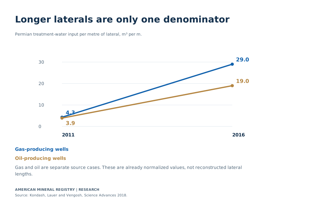
Did water input rise after accounting for horizontal lateral length?
The paper reports Permian injection intensity rising from 4.3 to 29.0 m³ per metre of lateral for gas-producing wells and from 3.9 to 19.0 m³ per metre for oil-producing wells between 2011 and 2016. AMR calculates increases of 574.4186% and 387.1795% respectively from those printed normalized values. Kondash and colleagues, Results, lateral-length discussion.

View chart data
Permian treatment-water input per metre of lateral, m3 per m.
| Source case | 2011 intensity (m3 per m) | 2016 intensity (m3 per m) |
|---|---|---|
| Gas-producing wells | 4.3 | 29.0 |
| Oil-producing wells | 3.9 | 19.0 |
Historical selected cases from Kondash et al. 2018, not current US averages.
Source-period and statistical definitions apply; AMR endpoint arithmetic does not reconstruct original uncertainty.
Kondash, Lauer and Vengosh, 2018, Results, Permian lateral-normalized values Kondash, Lauer and Vengosh 2018; Results paragraph 1, Permian gas/oil normalization sentences
| Permian source case | Start year | End year | Start injection intensity (m3 per m lateral) | End injection intensity (m3 per m lateral) | AMR endpoint multiple | AMR change (%) |
|---|---|---|---|---|---|---|
| Gas-producing wells | 2011 | 2016 | 4.3 | 29.0 | 6.7442 | 574.4186 |
| Oil-producing wells | 2011 | 2016 | 3.9 | 19.0 | 4.8718 | 387.1795 |
A horizontal lateral is the portion of the well extending through the target formation after the well turns from its vertical section. A longer lateral changes the scale of the completion. Water per well can therefore rise alongside a larger physical development footprint. Water per metre of lateral asks whether the treatment-water input also changed relative to that length. The two statistics describe related but distinct features of the operation.
In these reported Permian cases, the normalized input increased as well. The source’s evidence therefore supports more than a statement that the per-well quantity grew while wells became longer. It shows increased water input under the paper’s length-normalized measure. It does not, by itself, identify the contribution of every design change or establish a causal explanation for the entire difference.
AMR’s oil-case endpoint multiple is 19.0 / 3.9 = 4.8718. The gas-case multiple is 29.0 / 4.3 = 6.7442. These are calculations from source-normalized quantities. They are not estimates of the ratio between gas-well and oil-well lengths, nor a conversion between the two types of development.
Statistical order also matters. The ratio of two medians is not generally the same statistic as the median of individual ratios. The printed summary values do not authorize reconstructing a typical lateral length by dividing a median water volume by a separate normalized input. Such a calculation would require knowing that its inputs and aggregation procedure were compatible. This article uses the normalized values directly, as the source reports them.
The normalization comparison likewise supplies no freshwater fraction, water-quality result or current water requirement per metre. It answers a historical engineering-scale question within the named cases. Keeping that question explicit makes the metric useful without turning it into a measure of every consequence associated with water use.
Why is first-year wastewater not a fraction of the injected water returned?
The source’s FP measure combines returned injected fluid with formation water, while its injection and production summaries use different cohort clocks and statistical construction. Dividing the regional printed endpoints would not identify what fraction of the identical injected water came back from a matched well. Kondash and colleagues, Introduction, Results and Statistical methods.

View chart data
A schematic of the study method. No measured flow split or matched-well water balance is implied.
| Measure | Grouping clock | Statistic | Observation boundary |
|---|---|---|---|
| Injected treatment water | Spud year | Regional median input | Fracturing-water disclosure input |
| Flowback and produced water | First-production year | Sum of 12 monthly medians | Months 1 to 12 of production |
Historical selected cases from Kondash et al. 2018, not current US averages.
Source-period and statistical definitions apply; AMR endpoint arithmetic does not reconstruct original uncertainty.
Kondash, Lauer and Vengosh, 2018, Experimental design, Data acquisition and Statistical methods Kondash, Lauer and Vengosh 2018; Methods, Experimental design and Statistical methods
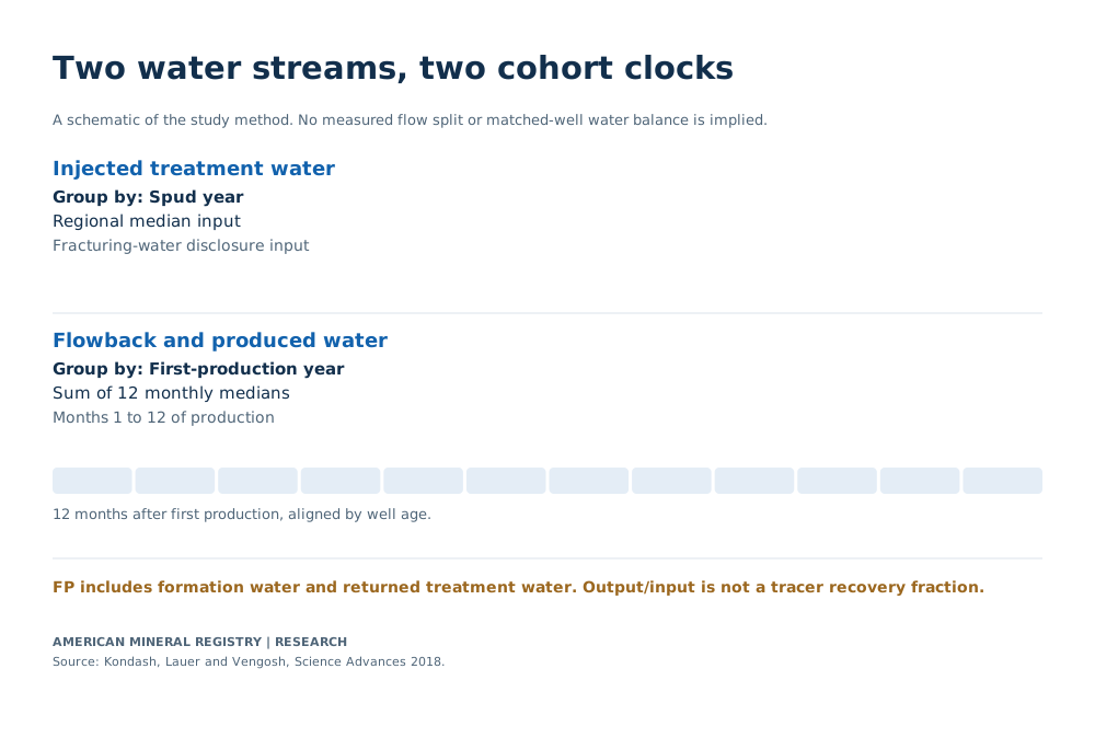
| Measure | Primary input named by study | Grouping clock | Published statistic construction | Unit and limit |
|---|---|---|---|---|
| Hydraulic-fracturing water use | FracFocus disclosure data, spatially assigned to producing region | Spud year | Median water-use value among source records in each region/spud year | m3 per well; does not identify freshwater fraction |
| First-year flowback and produced water | DrillingInfo production reports; PA DEP supplement for Marcellus | Year of first production, then month since first production | Median for each production month; first 12 monthly medians added for year-1 estimate | m3 per well for first 12 months; not a lifetime volume or matched tracer return fraction |
The physical issue comes first. Formation water is already present underground and can enter production alongside returned treatment water. The source explains that the contribution of saline formation water grows with time. An output-to-input volume comparison therefore includes an additional water source. It cannot serve as a tracer test of injected-fluid recovery without information separating those origins.
The paper itself describes Permian oil and gas FP-water-to-injection ratios above one. That observation is compatible with a mixed water stream that includes formation water. It should not be restated as more than 100% of the original injected water returning. The numerator and denominator describe different physical totals. Kondash and colleagues, Results, FP water to water-use ratio discussion.
The statistical issue is separate. Injection records are grouped by spud year, which identifies when drilling began. Production records are grouped by initial-production year and aligned by months since production started. A well’s drilling and production clocks need not fall into the same calendar grouping. The published regional summaries also do not establish that the precise same reporting wells contribute to both statistics.
For the first-year FP estimate, the source calculates monthly medians and adds the first 12 of them. That operation remains distinct from a median injection quantity and from a median of matched well-level return fractions. Dividing these summaries would introduce a new statistic. Its numerical result might look like a recovery fraction while lacking the physical and population boundaries required for that interpretation.
Coverage decisions further shape the comparison. The source removes area/year production data when DrillingInfo reporting is below 0.5% of its well-count denominator. It identifies Eagle Ford 2016 and Haynesville 2015 and 2016 exclusions, and replaces Marcellus 2015 and 2016 data with Pennsylvania DEP records. These are analysis rules, not observations that no production or wastewater existed in those areas and years. Kondash and colleagues, Statistical methods.
| Source rule or case | Specified period or threshold | Method action | Effect on this comparison |
|---|---|---|---|
| Minimum DrillingInfo reporting coverage | Below 0.5% of well-count denominator | Remove affected area/year data | Coverage screen, not proof of no production |
| Eagle Ford gas and oil | 2016 | Removed from DrillingInfo production analysis under coverage rule | FP endpoint comparison stops in 2015 |
| Haynesville | 2015 and 2016 | Removed from DrillingInfo production analysis under coverage rule | No reconstructed FP endpoint row supplied here |
| Marcellus | 2015 and 2016 | DrillingInfo replaced with Pennsylvania DEP records | Source change retained; no invented matched statewide panel |
| Bootstrap intervals | 95% intervals; 1000 resamples | Resample monthly empirical distributions; source describes error propagation | No new uncertainty interval calculated from rounded main-text endpoints |
The useful inference concerns management scale: the study documents larger early wastewater quantities in its reported cases. It does not establish the origin of every litre, the share reused, the fraction disposed by any particular route or the lifetime water outcome of a well. Those questions require their own measured quantities and observation boundaries.
How does the answer change when water use is divided by energy output?
For the Permian oil case, the paper reports water-use intensity of 11 L/GJ in 2011 and 28 L/GJ in 2016, using hydrocarbon energy from the first 12 production months. AMR calculates a 154.5455% increase from those printed values. This uses a different denominator from either water per well or water per metre of lateral. Kondash and colleagues, Results, water-use intensity discussion and Fig. 4.

View chart data
Permian oil water-use intensity, litres per GJ of first-year hydrocarbon energy.
| Source case | 2011 intensity (L per GJ) | 2016 intensity (L per GJ) |
|---|---|---|
| Permian oil | 11 | 28 |
Historical selected cases from Kondash et al. 2018, not current US averages.
Source-period and statistical definitions apply; AMR endpoint arithmetic does not reconstruct original uncertainty.
Kondash, Lauer and Vengosh, 2018, Results and Statistical methods, energy conversion Kondash, Lauer and Vengosh 2018; Results paragraph 5; Fig.4; Methods energy assumptions
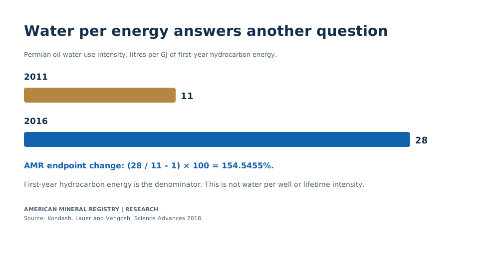
| Source case | Start year | End year | Start water-use intensity (L per GJ) | End water-use intensity (L per GJ) | AMR endpoint multiple | AMR change (%) | Energy window |
|---|---|---|---|---|---|---|---|
| Permian oil | 2011 | 2016 | 11 | 28 | 2.5455 | 154.5455 | Hydrocarbon energy generated during first 12 months; source conversion assumptions apply |
Water per unit of energy asks how a treatment-water input compares with a specified production output. If both water input and hydrocarbon output change, the normalized measure can change differently from the per-well quantity. The difference is expected because the denominator has changed. A smaller percentage increase in a normalized metric does not mean that the additional per-well water disappeared.
The source converts oil and gas volumes into energy using stated energy-content assumptions. Its calculations for gas-producing and oil-producing wells also account for associated hydrocarbon streams under that method. The resulting L/GJ values therefore carry both an observation-window condition and a conversion-model condition. They should be attributed to the study, rather than presented as a direct physical measurement of the entire energy life cycle.
The first-year window is particularly important for an energy comparison. Later hydrocarbon output and later produced water lie outside the displayed early-production denominator. A lifetime intensity would need a compatible lifetime production estimate and an explicit treatment of the water numerator. AMR does not extend the source’s first-year values into a lifetime ratio.
This distinction also prevents cross-sector comparisons from acquiring an accidental meaning. Water per GJ of early hydrocarbon production, water used to generate electricity and water consumed over a full fuel cycle can describe different stages and types of water accounting. Matching units alone does not make their system boundaries identical. This reference keeps the question inside the source’s treatment-input and first-year-production framework.
The metric dictionary below states the numerator and denominator for each principal quantity. The finding-input table provides the exact expressions behind AMR’s reusable calculations. Readers can select a statistic for their question while preserving the source case, dates and essential qualification.
| Metric | Numerator | Denominator or boundary | What it can support | Unsupported substitution |
|---|---|---|---|---|
| Injection per well | Hydraulic-fracturing treatment water | Source well statistic grouped by spud year | A regional per-well input comparison | Freshwater consumption, all drilling water or basin total |
| First-year FP per well | Combined flowback and produced water | First 12 production months by initial-production cohort | A historical early wastewater-management comparison | Lifetime water production or injected-water return fraction |
| Injection per lateral length | Treatment-water volume | Metres of horizontal lateral | Source-normalized input comparison | Proof that lateral growth alone explains change |
| Water-use energy intensity | Treatment-water volume | Hydrocarbon energy during first 12 months, with source conversions | Source water-per-energy comparison | Plant electricity water use, lifetime intensity or national average |
| FP water to injection ratio | Combined formation and returned treatment water | Injected treatment-water volume within source analysis | Comparison of mixed water output and input | Fraction of the identical injected water recovered |
| Finding | Input expression | AMR result | Unit | Source boundary |
|---|---|---|---|---|
| Permian injection change | (42500 / 4900 - 1) * 100 | 767.3469 | Percent | 2011 to 2016 printed median injection endpoints |
| Eagle Ford gas first-year FP change | (20700 / 1340 - 1) * 100 | 1444.7761 | Percent | 2011 to 2015 first-production cohorts; first 12 months |
| Permian oil lateral-normalized change | (19.0 / 3.9 - 1) * 100 | 387.1795 | Percent | 2011 to 2016 source-normalized injection input |
| Permian oil energy-normalized change | (28 / 11 - 1) * 100 | 154.5455 | Percent | 2011 to 2016; first-year hydrocarbon energy boundary |
How should these statistics be quoted?
Keep the historical period, basin or production case, unit and observation window in the sentence. For example: “From the 2018 study’s printed Permian injection medians, AMR calculates a 767.3469% increase between 2011 and 2016.” For FP water, add “combined flowback and produced water during the first 12 production months” and retain the actual cohort endpoint. Credit the original authors for the study and AMR for the stated recomputation.
Frequently asked questions
Is there one current US water-per-fracked-well number on this page?
This comparison concerns named historical source cases. A current national estimate would need current coverage, consistent definitions and a specified method for combining wells and regions. The older endpoint quantities do not establish that estimate.
Does injected water equal freshwater consumption?
Injection volume, source-water type, withdrawal and net consumption describe different quantities. The printed treatment-water endpoints do not supply the freshwater share or a complete water-source accounting. Retain the injection label instead of substituting an unsupported freshwater quantity.
Does produced water mean only the injected water that came back?
The paper’s FP measure combines returned treatment water and formation water. A recovery fraction for the original injected fluid requires an origin-specific, matched measurement. An aggregate output-to-input ratio does not provide it. Kondash and colleagues, Introduction and Results.
Why does Eagle Ford stop at 2015 while other rows reach 2016?
The paper’s production analysis removes the 2016 Eagle Ford gas and oil records under its reporting-coverage rule. Its printed first-year endpoint comparison therefore stops with the 2015 cohort. The overall study window should not replace that case-specific year. Kondash and colleagues, Statistical methods.
Can the regional median be multiplied by a well count to get total use?
That would create a new estimate with a particular aggregation assumption. A median is not generally the mean required to reconstruct a total by simple multiplication. A defensible total needs compatible observations or a stated model, appropriate counts and consistent coverage.
Do the extra decimal places establish precise original measurements?
They express AMR’s arithmetic from the displayed source endpoints. The physical source values are rounded and have statistical uncertainty. AMR does not infer a new confidence interval or recover unrounded data by adding decimal places.
Does this comparison validate the paper’s projections through 2030?
The article examines historical endpoint observations and source methods. Projections require their own assumptions and outcome evaluation. No future scenario is presented here as an observed result.
Methodology and Sources
The primary source is Kondash, Lauer and Vengosh’s 2018 Science Advances paper, “The intensification of the water footprint of hydraulic fracturing”, DOI 10.1126/sciadv.aar5982. AMR inspected its accessible full main text, source figure captions and methods. The numerical comparison is deliberately limited to complete endpoint cases explicitly printed there, with compatible definitions retained per table.
AMR transcribed the injection endpoints in Results paragraph 1, the first-year FP endpoints in paragraph 2, the Permian lateral-normalized inputs in paragraph 1 and the Permian oil energy-normalized inputs in paragraph 5. The coverage and cohort ledger follows the source’s Experimental design, Data acquisition and Statistical methods. No missing annual observations, basin rows or uncertainty limits were reconstructed from chart pixels or neighboring cases.
Changes are calculated as later minus earlier for absolute differences and (later / earlier − 1) × 100 for percentage increases. Endpoint multiples divide later by earlier. Published percentage summaries remain separate from AMR recomputations using rounded printed volumes. The source-cell ledger identifies every displayed cell, primary URL, source paragraph and calculation. The standalone reproduction program reads the matching CSVs and verifies these operations, endpoint windows and essential source inputs.
The original study uses DrillingInfo production data alongside public sources and describes bootstrap uncertainty and coverage screening. AMR’s reproduction covers its own displayed-input calculations, rather than a full rebuild of the original well-level analysis. It does not estimate new confidence intervals, establish an injected-fluid return fraction, measure freshwater consumption or update the historical observations to current conditions.
Glossary
- Hydraulic-fracturing water input. Treatment-water volume reported under the source’s injection analysis, distinct from all water used over the full development life cycle.
- Flowback and produced water, FP. The source’s combined water stream containing returned injected fluid and formation water.
- Formation water. Water present underground that can enter a producing well alongside hydrocarbons.
- Spud year. The year drilling began, used to group the source’s injection records.
- First-production cohort. Wells grouped by the year production started, then aligned by months since first production.
- Year-one estimate. The source’s sum of the first 12 monthly production medians, with its described uncertainty method.
- Lateral. The horizontal portion of a well extending through the target formation.
- Median. The central ranked observation, which need not equal the mean or reproduce a population total.
- Water-use intensity. A source-defined water input divided by a specified output or physical scale, with the denominator stated.
- Percentage point. The arithmetic difference between two percentages, distinct from a percentage change in a physical volume.
Sources
- Kondash, A. J., Lauer, N. E. and Vengosh, A. The intensification of the water footprint of hydraulic fracturing. Science Advances 4, eaar5982, 2018. Primary historical observations and methods. Main locations: Results paragraphs 1, 2, 5 and 6; Figs. 2 to 4 captions; Materials and Methods, Experimental design, Data acquisition and Statistical methods.
- Persistent article DOI. DOI identity for the same primary work. AMR’s contribution is the explicitly labeled endpoint arithmetic, source-window reconciliation and denominator dictionary.