This reference follows the same ten counties through fifteen years, compares them with all 254 Texas counties, and explains the income, population and ranking calculations. The group comes from a published preliminary oil production table, rather than a search for counties with high incomes. Complete tables, original definitions and reproducible downloads preserve the comparison and its limits.
Key Takeaways
- Eight of ten fixed oil cohort counties exceeded Texas personal income per resident in 2024. (AMR calculations from BEA, Feb 2026).
- The cohort's combined 2024 personal income per resident was $123,442. (AMR calculations from BEA, Feb 2026).
- The unweighted median of the ten county PCPI figures was $90,529 in 2024. (AMR calculations from BEA, Feb 2026).
- Texas reported per capita personal income of $69,823 in 2024. (BEA CAINC1, Feb 2026).
- Loving reported $220,625 per resident in 2024, using a population of 48. (BEA CAINC1, Feb 2026).
- Midland reported $146,414 per resident and ranked third among Texas counties in 2024. (AMR calculations from BEA, Feb 2026).
- The fixed ten counties contained 273,083 residents in 2024. (AMR calculations from BEA, Feb 2026).
- The cohort represented 0.8727% of Texas population and 1.5429% of Texas personal income in 2024. (AMR calculations from BEA, Feb 2026).
- Midland accounted for 67.23% of cohort population and 79.74% of cohort personal income in 2024. (AMR calculations from BEA, Feb 2026).
- Combined cohort personal income per resident increased 114.1% in nominal terms from 2010 through 2024. (AMR calculations from BEA, Feb 2026).
- The cohort population increased 19.8% from 2010 through 2024, with different paths across counties. (AMR calculations from BEA, Feb 2026).
- Reeves moved from Texas PCPI rank 248 in 2010 to rank 26 in 2024. (AMR calculations from BEA, Feb 2026).
- Eight selected counties improved their Texas PCPI ranks from 2010 through 2024; two moved lower. (AMR calculations from BEA, Feb 2026).
- The fixed cohort follows January 2024 preliminary crude oil production, excluding separately reported condensate. (Railroad Commission of Texas, Apr 2024).
Which Texas oil counties had higher income per resident in 2024?
Most counties in this fixed group exceeded the state figure, but the range was wide. Keeping every selected county visible prevents the high values in a few small counties from becoming a claim that all oil producing counties have similar incomes.

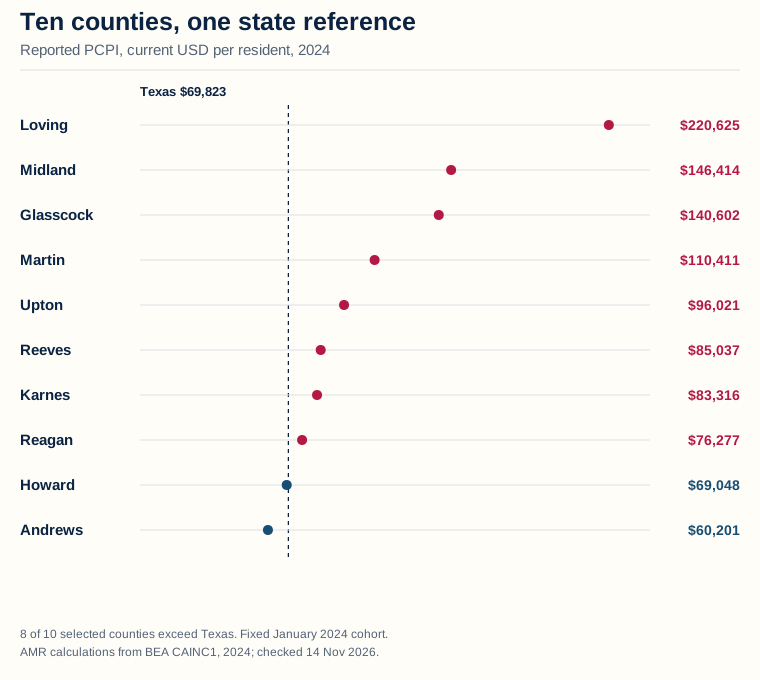
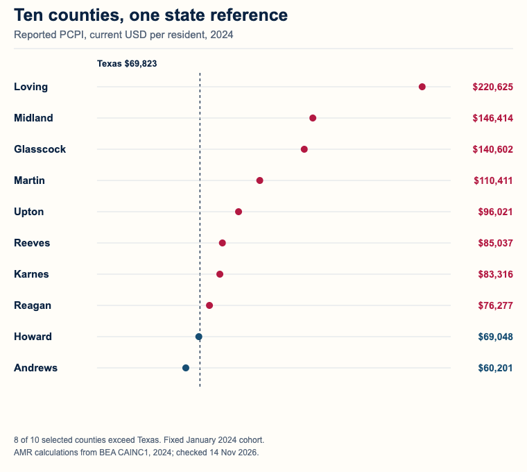
Figure 1 in text
Which counties exceed the state? 2024 Texas oil-county income statistics: eight of ten fixed-cohort counties exceeded Texas per capita personal income of $69,823.
Ten counties, one state reference Reported PCPI, current USD per resident, 2024
Texas $69,823
Loving
$220,625
Midland
$146,414
Glasscock
$140,602
Martin
$110,411
Upton
$96,021
Reeves
$85,037
Karnes
$83,316
Reagan
$76,277
Howard
$69,048
Andrews
$60,201 8 of 10 selected counties exceed Texas. Fixed January 2024 cohort. AMR calculations from BEA CAINC1, 2024; checked 14 Nov 2026.
Additional phone figure text: Ten counties versus Texas · 8 of 10 counties exceed Texas. Fixed oil cohort. · AMR from BEA CAINC1, 2024. 14 Nov 2026.
Source and data: BEA, CAINC1 county personal income summary
Permanent link to this figure’s text and data · Sources and context
Which selected counties had the highest figures?
Loving, Midland and Glasscock occupied the first three positions within the group. They also had high positions in the complete Texas county comparison, although their population sizes were very different.
Loving's reported 2024 per capita personal income, or PCPI, was $220,625, the highest among all 254 Texas counties in this pinned BEA file. Midland reported $146,414 and ranked third statewide. Glasscock reported $140,602 and ranked fourth. These are income per resident figures, with the state rank calculated across counties rather than across households or individuals. (AMR calculations from BEA, Feb 2026).
The next three selected counties were Martin at $110,411, Upton at $96,021 and Reeves at $85,037. Their Texas ranks were 12, 19 and 26 respectively. County identity remains fixed in this study; their income order is an analytical result, rather than the criterion used to select them. (AMR calculations from BEA, Feb 2026).
The complete comparison below uses the source's reported whole dollar PCPI for both county ranks and ratios to Texas. The downloadable data also retain the quotient calculated directly from personal income and population, so rounding can be inspected rather than hidden.
| County | Reported PCPI, USD, 2024 | Texas rank of 254 | Ratio to Texas | Population, 2024 |
|---|---|---|---|---|
| Loving | 220,625 | 1 | 3.160 | 48 |
| Midland | 146,414 | 3 | 2.097 | 183,587 |
| Glasscock | 140,602 | 4 | 2.014 | 1,153 |
| Martin | 110,411 | 12 | 1.581 | 5,179 |
| Upton | 96,021 | 19 | 1.375 | 3,128 |
| Reeves | 85,037 | 26 | 1.218 | 11,956 |
| Karnes | 83,316 | 28 | 1.193 | 15,137 |
| Reagan | 76,277 | 40 | 1.092 | 3,139 |
| Howard | 69,048 | 65 | 0.989 | 30,833 |
| Andrews | 60,201 | 113 | 0.862 | 18,923 |
Source: AMR calculations from BEA CAINC1, Feb 2026. Ratios rounded to three decimal places. Download all ten comparison rows (CSV).
How far above or below Texas were the counties?
The state comparison provides a consistent reference point, while preserving the fact that Texas includes these same counties. A ratio above one indicates a higher county PCPI than the state's reported PCPI for the same year.
Loving's 2024 figure was approximately 3.160 times Texas PCPI. Midland's was approximately 2.097 times, and Glasscock's approximately 2.014 times. These ratios compare area averages; they do not mean that every resident earned the corresponding multiple of a state resident's income. (AMR calculations from BEA, Feb 2026).
Howard's $69,048 was slightly below Texas's $69,823, yielding a ratio of approximately 0.989. Andrews's $60,201 yielded approximately 0.862. Retaining both counties is essential: an account that shows only counties above Texas would change the selected group after seeing the answer. (AMR calculations from BEA, Feb 2026).
The state benchmark is an average across the population, not the median Texas county. It should therefore be described as the Texas PCPI figure. Calling it the income of the typical county, household or worker would substitute a different statistic without evidence.
Why compare with all 254 Texas counties?
A complete state comparison makes the rank meaningful. Ranking only the ten selected places would answer who is highest within this group, while leaving their position in Texas unclear.
The working panel includes every one of the 254 Texas counties for every year from 2010 through 2024, giving 3,810 county and year observations. Texas's own state observations are retained separately. The source gate verified personal income, population and reported PCPI for all selected years and geographies before the article was drafted. (AMR calculations from BEA, Feb 2026).
A rank is calculated as one plus the number of Texas counties with a strictly higher reported PCPI. Equal published values share a rank, and subsequent positions retain the corresponding gap. This competition ranking rule prevents an arbitrary county name sort from breaking a tie.
The comparison is deliberately bounded to Texas. It is not a national county ranking, a census of every oil community, or a result for every county in the Permian Basin. The complete state table supports the claim being made without requiring unsupported national coverage.
What does per capita personal income actually measure?
PCPI divides an area's total personal income by its resident population. Understanding that numerator and denominator is necessary before turning a striking county value into a headline about salaries, households, wealth or mineral royalties.

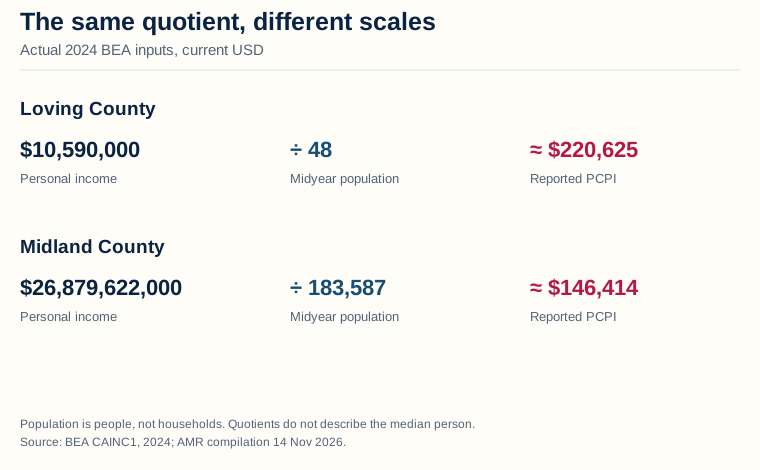
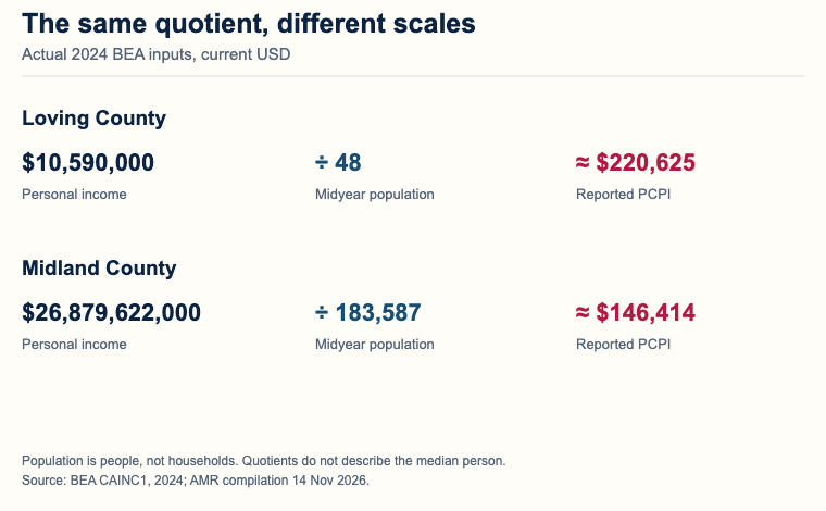
Figure 2 in text
What does the denominator change? Actual 2024 BEA income and population: Loving $10.590million/48 residents=$220625; Midland $26.879622billion/183587 residents≈$146414.
The same quotient, different scales Actual 2024 BEA inputs, current USD
Loving County
$10,590,000
÷ 48
≈ $220,625 Personal income Midyear population Reported PCPI
Midland County
$26,879,622,000
÷ 183,587
≈ $146,414 Personal income Midyear population Reported PCPI Population is people, not households. Quotients do not describe the median person. Source: BEA CAINC1, 2024; AMR compilation 14 Nov 2026.
Additional phone figure text: Income divided by residents · $10,590,000 personal income · ÷ 48 residents · = $220,625 per resident · $26,879,622,000 personal income · ÷ 183,587 residents · ≈ $146,414 per resident · People, not households. Values rounded by BEA. · Source: BEA CAINC1, 2024; AMR 14 Nov 2026.
Source and data: BEA, CAINC1 definitions and county estimates
Permanent link to this figure’s text and data · Sources and context
What income and population enter the calculation?
The income concept is broader than wages, and the population concept is broader than workers. BEA's source definitions describe income received by or on behalf of people who reside in the area.
Personal income includes wages and salaries, employer supplements, proprietors' income, rental income, dividends, interest and current transfer receipts, with the source's specified adjustments. Consequently, county PCPI cannot be treated as average employee pay. A change can reflect several forms of income even when the number of local jobs is unchanged. (BEA, CAINC1 definitions, Feb 2026).
The population denominator is the resident population. BEA's footnote specifies Census Bureau midyear population estimates, including people who are not employed. Children, retired residents and other residents remain part of the denominator; the table does not divide by the number of oil workers. (BEA, CAINC1 footnotes, Feb 2026).
BEA's personal income concept also includes some noncash income, such as employer contributions for insurance. Its learning material excludes capital gains from stock price changes. Neither annual income nor its per resident quotient is a balance sheet measure of assets minus liabilities. (BEA, Income and Saving, checked Nov 2026).
The calculation program multiplies CAINC1 personal income by 1,000 before dividing by population because the income line is supplied in thousands of dollars. Omitting that conversion would make the resulting dollar figure one thousand times too small.
Why can a small population produce a striking figure?
The same arithmetic applies to every county, but an exceptionally small denominator makes the resulting average sensitive to changes in either total income or population. The published inputs should accompany an exceptional quotient.
Loving's 2024 personal income was $10,590,000 and its population was 48. Dividing those exact source inputs gives $220,625 per resident. This is a verified quotient of area totals, rather than evidence that a median Loving household or every Loving resident received $220,625. (AMR calculations from BEA, Feb 2026).
Midland's personal income was $26,879,622,000 and its population was 183,587. The quotient is approximately $146,413.54 per resident; BEA's reported whole dollar PCPI is $146,414. Thus Midland has the lower per resident figure of the pair while having the much larger total income. (AMR calculations from BEA, Feb 2026).
A county rank alone removes both of those dimensions. Including the income total and population lets readers distinguish a small place with an exceptional quotient from a populous area accounting for a large share of regional income. It also gives another researcher the actual inputs needed to reproduce the result.
No household distribution is present in CAINC1. A high quotient could coexist with unequal incomes, but this table does not measure that inequality. Quantifying it would require a separately sourced distribution, with a compatible population, income concept and period.
Is PCPI the same as median household income or take home pay?
It is neither. A per resident quotient, a middle household value and income after taxes use different concepts and denominators, so their labels cannot be exchanged even when their dollar values appear comparable.
The median of the ten county PCPIs is a median across ten area averages. It is not the median income of the residents living across those counties. The middle two county figures determine that statistic even though the counties have different numbers of residents.
Similarly, county personal income is not disposable personal income. BEA defines disposable personal income as the income remaining after personal taxes. The CAINC1 income and PCPI lines used here do not apply that after tax transformation. (BEA, Income and Saving, checked Nov 2026).
The geography follows residence rather than simply the location of production or employment. BEA describes local income as including income of residents whose work takes place outside the area. A worker commuting into an oil county and a mineral owner living elsewhere are reasons to keep production geography and resident income conceptually separate; this study does not estimate either flow. (BEA, local personal income, checked Nov 2026).
For a household affordability story, a separately sourced household income and cost measure may be more appropriate. This article provides the full area income comparison while preserving what its underlying source can actually answer.
What is the income of the ten counties combined?
Adding the counties' personal income and dividing by their combined population produces one income per resident for the whole group. It differs from taking the mean or median of the ten published county values, because the weights differ.

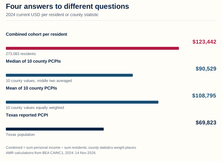
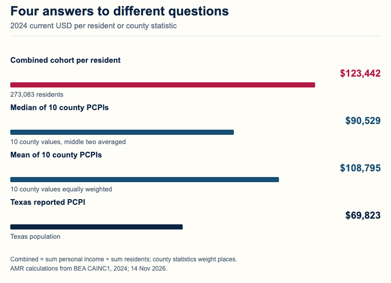
Figure 3 in text
Which cohort summary should a writer use? Four2024 measures:combined$123442,median$90529,mean$108795,Texas$69823. Different denominators are shown.
Four answers to different questions 2024 current USD per resident or county statistic
Combined cohort per resident
$123,442 273,083 residents
Median of 10 county PCPIs
$90,529 10 county values, middle two averaged
Mean of 10 county PCPIs
$108,795 10 county values equally weighted
Texas reported PCPI
$69,823 Texas population Combined = sum personal income ÷ sum residents; county statistics weight places. AMR calculations from BEA CAINC1, 2024; 14 Nov 2026.
Additional phone figure text: Combined uses all 273,083 residents. · County median/mean treat counties equally. · AMR from BEA CAINC1, 2024; 14 Nov 2026.
Source and data: BEA, CAINC1 county and state data
Permanent link to this figure’s text and data · Sources and context
Which number describes the combined resident population?
The combined quotient uses every resident in the selected counties through their source population totals. It does not give a county with a few dozen residents the same weight as one with hundreds of thousands.
The ten counties had $33,709,927,000 in combined personal income and 273,083 residents in 2024. Their quotient is $123,442.0561 per resident, or $123,442 rounded to the nearest dollar. AMR calculates this from the underlying totals rather than averaging rounded county PCPIs. (AMR calculations from BEA, Feb 2026).
That quotient was approximately 1.768 times Texas's reported $69,823 PCPI. It is a useful comparison of income per resident in the combined geography with the state, while preserving the fact that the state contains the selected geography. It does not describe a counterfactual Texas without oil production. (AMR calculations from BEA, Feb 2026).
Using the source totals also avoids a small rounding discrepancy. A population weighted average of the published whole dollar county PCPIs is an approximation to the quotient of total income and population. The article's combined measure uses the latter, and the CSV makes that choice explicit.
The reader can therefore use a precise description: combined personal income per resident for the fixed ten county group. Describing it merely as average oil county income would leave both the included counties and the weighting rule unclear.
Why do the county mean and county median give different answers?
They answer questions about the set of counties rather than directly describing the combined resident population. Each county contributes one value regardless of its population.
The unweighted median of the ten reported county PCPIs was $90,529 in 2024. It is the mean of the fifth and sixth ordered values, $96,021 in Upton and $85,037 in Reeves. Those two figures determine the median even though neither is the cohort's combined per resident quotient. (AMR calculations from BEA, Feb 2026).
The unweighted arithmetic mean was $108,795.20. Every county's reported PCPI receives one tenth of the weight in that calculation, so Loving and Midland each count once despite their different resident populations. The difference from the $123,442.0561 combined quotient follows from weighting and the source values, rather than an error that requires one statistic to be discarded. (AMR calculations from BEA, Feb 2026).
For a story about the middle county, use the county median and name the ten county selection. For a story about income per resident across the selected geography, use the combined quotient. For a story about a typical household, neither supplies the required household distribution.
The complete weighting table (CSV) provides all three statistics for each of the fifteen years. It lets a writer maintain one definition through a time comparison rather than quietly switching to whichever summary appears more striking in each year.
How much does Midland influence the combined result?
Midland accounts for a substantial majority of the group's residents and personal income. Showing that concentration explains why the combined quotient can sit well above the median county figure.
Midland represented 67.23% of the cohort's 273,083 residents in 2024, using its population of 183,587. It accounted for 79.74% of the group's $33.709927 billion personal income total, using Midland's $26.879622 billion. The two percentages have separate denominators and describe concentration within the fixed cohort. (AMR calculations from BEA, Feb 2026).
Loving, despite its first ranked PCPI, contributed only 48 residents to the combined population. Its high county quotient does not receive equal population weight in the combined measure. Keeping both observations visible prevents a visually dramatic small county from being mistaken for the principal source of the cohort's aggregate income. (AMR calculations from BEA, Feb 2026).
Concentration also affects interpretation of change. A movement in Midland's income can move the combined quotient substantially, while a movement in a small county can strongly change that county's rank with little effect on the combined total. Neither pattern identifies what caused the underlying income movement.
The county concentration download supplies each selected county's income and population shares, rather than leaving the Midland comparison as an isolated calculation. Its totals reconcile with the same cohort totals used throughout the article.
How did the fixed cohort change from 2010 through 2024?
The combined cohort remained above Texas PCPI across the selected years, but the size of the difference changed. A complete annual series reveals declines and recoveries that a single starting and ending comparison would conceal.

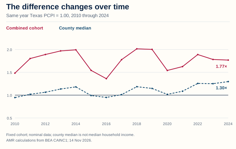
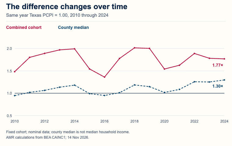
Figure 4 in text
Did the income difference persist? Income ratios to Texas,2010through2024:combined cohort remains above1.00;county median varies around and above parity.
The difference changes over time Same year Texas PCPI = 1.00, 2010 through 2024
Combined cohort
County median 0.5 1.0 1.5 2.0
1.77×
1.30× 2010 2012 2014 2016 2018 2020 2022 2024 Fixed cohort; nominal data; county median is not median household income. AMR calculations from BEA CAINC1; 14 Nov 2026.
Additional phone figure text: Fixed cohort and source vintage. Nominal data.
Source and data: BEA, CAINC1 annual history
Permanent link to this figure’s text and data · Sources and context
Was the cohort always above the state figure?
The answer depends on which cohort summary is being compared. The weighted combined measure and the unweighted county median should remain distinct throughout the history.
Combined cohort personal income per resident was approximately $57,663 in 2010, compared with Texas's $38,911, a ratio of approximately 1.482. In 2024, the corresponding figures were approximately $123,442 and $69,823, a ratio of approximately 1.768. The combined quotient exceeded Texas in every included year. (AMR calculations from BEA, Feb 2026).
The county median began at $36,846.50 in 2010, below Texas's $38,911. It reached $90,529 in 2024, above Texas's $69,823. A statement that the median county always exceeded Texas would therefore be false for this fixed sample and window. (AMR calculations from BEA, Feb 2026).
The number of selected counties exceeding Texas also changed. It was four in 2010, three in 2016, nine in 2022 and eight in 2024. Those counts compare each county with that year's state PCPI, using the same ten counties throughout. (AMR calculations from BEA, Feb 2026).
These differences make the whole annual history useful. The combined quotient can remain above Texas while fewer than half of the selected counties individually exceed Texas, because residents are not distributed evenly across the counties.
How much of the increase was income growth and how much was population change?
Income per resident is a ratio. Its growth follows the growth of the income numerator relative to the growth of the population denominator, rather than the income growth percentage alone.
From 2010 through 2024, the cohort's personal income increased from $13.148228 billion to $33.709927 billion, a nominal increase of 156.4%. Population increased from 228,018 to 273,083, or 19.8%. The resulting combined income per resident increased 114.1%. (AMR calculations from BEA, Feb 2026).
The precise identity is: the ending income divided by starting income, divided by the ending population divided by starting population, equals the ending income per resident divided by starting income per resident. Multiplying that last ratio minus one by 100 expresses the per resident percentage change.
Subtracting the population growth percentage from the income growth percentage would not reproduce the exact result. That shortcut neglects the ratio relationship, particularly when changes are substantial. The downloadable growth table retains the multiplicative factors as well as percentages for each selected county.
All dollar comparisons here are nominal. BEA's source footnote specifies current dollars, without an inflation adjustment. The 114.1% result therefore does not establish a 114.1% increase in purchasing power, and no county cost of living adjustment is implied. (BEA CAINC1 footnotes and AMR calculations, Feb 2026).
What would an endpoint comparison miss?
A start and end increase does not describe the path between those years. It can coexist with sizeable intermediate decreases, changes in relative standing and different patterns across counties.
The combined quotient was approximately $93,138 in 2014, $72,125 in 2015 and $62,411 in 2016. It later reached approximately $106,663 in 2019 before declining to approximately $84,464 in 2020. These nominal annual observations illustrate why the full series should accompany a long period growth claim. (AMR calculations from BEA, Feb 2026).
The combined cohort to Texas ratio was approximately 1.992 in 2014, 1.361 in 2016, 2.014 in 2018 and 1.768 in 2024. A higher ending dollar value does not require an uninterrupted rise in the ratio to the state. Texas's own income per resident changes in the same comparison. (AMR calculations from BEA, Feb 2026).
The source and this calculation do not isolate why any particular annual change occurred. Assigning it to oil prices, employment, royalties, transfers or migration would require additional components and an appropriate analytical design. The time series establishes the change, rather than a causal decomposition of its economic drivers.
For a separate view of commodity movements, the winter gas prices and monthly volatility reference analyzes wholesale benchmarks. Those prices should not be substituted for the resident income observations on this page.
Did every county gain income, population and rank?
The counties did not follow a uniform path. A county can gain nominal income per resident while losing population, and it can gain income per resident while moving lower in the state ranking if other counties gain more.

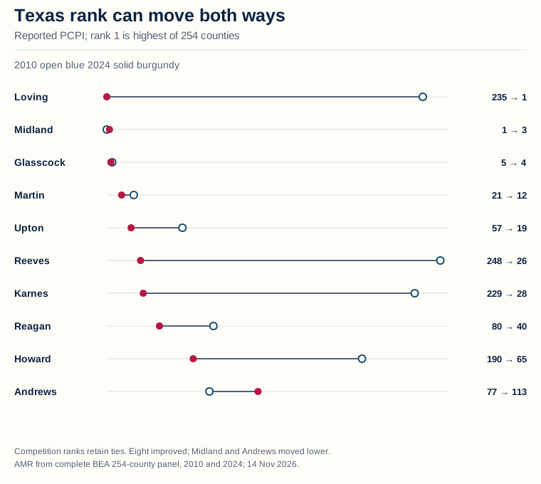
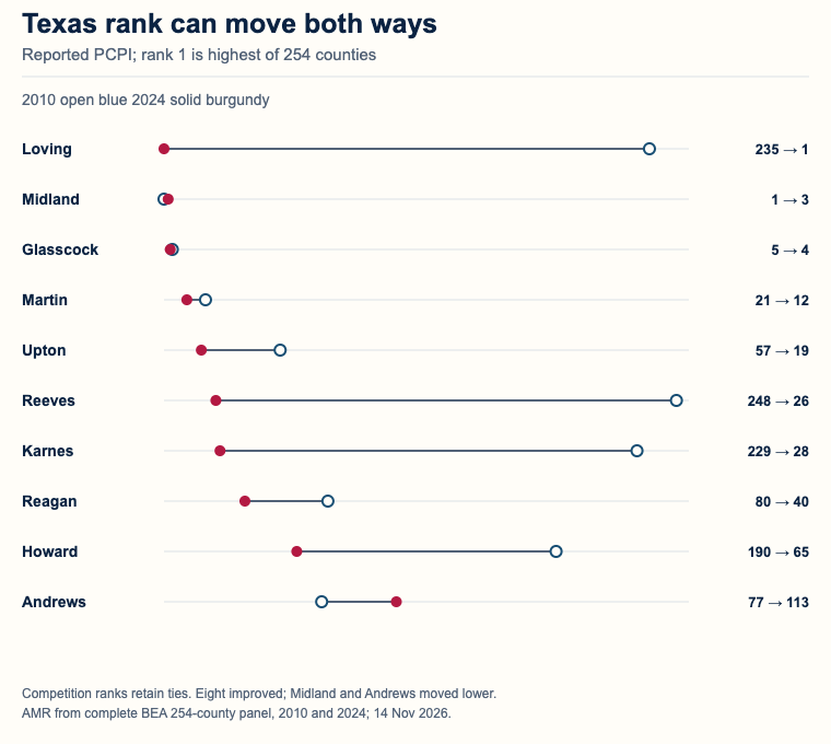
Figure 5 in text
Did every county move the same way? Texas PCPI ranks2010to2024:Reeves248to26,Loving235to1,Karnes229to28;Midland1to3,Andrews77to113.
Texas rank can move both ways Reported PCPI; rank 1 is highest of 254 counties 2010 open blue 2024 solid burgundy
Loving
235 → 1
Midland
1 → 3
Glasscock
5 → 4
Martin
21 → 12
Upton
57 → 19
Reeves
248 → 26
Karnes
229 → 28
Reagan
80 → 40
Howard
190 → 65
Andrews
77 → 113 Competition ranks retain ties. Eight improved; Midland and Andrews moved lower. AMR from complete BEA 254-county panel, 2010 and 2024; 14 Nov 2026.
Additional phone figure text: Eight improved; two moved lower. Ties retained. · AMR from BEA 254-county panel; 14 Nov 2026.
Source and data: BEA, CAINC1 complete Texas county panel
Permanent link to this figure’s text and data · Sources and context
Which counties moved most in the Texas ranking?
Ranks compare a county with all the other counties in the same year. They therefore add a relative dimension to the dollar changes, while retaining the source's published whole dollar PCPI for consistency.
Loving moved from rank 235 in 2010 to rank 1 in 2024. Reeves moved from rank 248 to rank 26, and Karnes moved from rank 229 to rank 28. Howard moved from rank 190 to rank 65. These are changes in the statewide income per resident ranking, not changes in production rank. (AMR calculations from BEA, Feb 2026).
Midland moved from first to third, while Andrews moved from rank 77 to rank 113. Both experienced positive nominal income per resident growth over the period. The result illustrates why falling in a ranking cannot by itself be reported as a fall in the underlying dollar measure. (AMR calculations from BEA, Feb 2026).
Rank changes do not have a dollar unit. Moving twenty positions in one part of a distribution need not represent the same dollar change as moving twenty elsewhere. The complete PCPI values and growth factors remain necessary for a meaningful comparison of magnitude.
| County | Texas rank, 2010 | Texas rank, 2024 | Personal income change, % | Population change, % | Calculated income per resident change, % |
|---|---|---|---|---|---|
| Andrews | 77 | 113 | 107.9 | 27.5 | 63.1 |
| Glasscock | 5 | 4 | 153.9 | minus 5.8 | 169.6 |
| Howard | 190 | 65 | 102.7 | minus 11.8 | 129.7 |
| Karnes | 229 | 28 | 216.6 | 1.8 | 210.9 |
| Loving | 235 | 1 | 409.9 | minus 40.7 | 760.4 |
| Martin | 21 | 12 | 165.7 | 8.0 | 146.0 |
| Midland | 1 | 3 | 160.9 | 34.2 | 94.4 |
| Reagan | 80 | 40 | 94.9 | minus 6.0 | 107.4 |
| Reeves | 248 | 26 | 221.3 | minus 13.4 | 270.8 |
| Upton | 57 | 19 | 130.6 | minus 6.1 | 145.7 |
Source: AMR calculations from BEA CAINC1, Feb 2026. Period 2010 through 2024; current dollars, no inflation adjustment. Growth uses unrounded income and population quotients. Download exact values and factors (CSV).
Can income per resident rise while population declines?
Yes. The quotient rises whenever the income numerator grows relative to the population denominator. That relationship does not require population growth, and it should not be interpreted as evidence that remaining residents all experienced the same increase.
Reeves's personal income increased 221.3% from 2010 through 2024 while its population decreased 13.4%. Calculated personal income per resident increased 270.8%. The larger per resident increase follows from a larger numerator divided by a smaller denominator. (AMR calculations from BEA, Feb 2026).
Glasscock's personal income increased 153.9% while population decreased 5.8%, producing a 169.6% increase in its calculated income per resident. Howard's income increased 102.7%, population decreased 11.8%, and calculated income per resident increased 129.7%. All percentages use the same start and end years. (AMR calculations from BEA, Feb 2026).
Loving is especially sensitive to this denominator issue. Its population decreased 40.7% while personal income increased 409.9%, yielding a 760.4% increase in the calculated quotient. The exact source populations are required to understand that result; a percentage growth headline without them would hide the scale of the place being described. (AMR calculations from BEA, Feb 2026).
These are accounting identities based on area totals. They do not establish whether the same people remained in the county or identify who received the additional income. The article does not infer individual mobility from repeated county aggregates.
What changes when population grows as well?
When both income and population grow, part of the increase in total income accompanies a larger resident population. The per resident measure divides the two growth factors rather than assigning the whole income increase to each resident.
Midland's personal income increased 160.9% and its population increased 34.2% from 2010 through 2024. Calculated income per resident increased 94.4%. Andrews's personal income increased 107.9% and population increased 27.5%, yielding a 63.1% increase in calculated income per resident. (AMR calculations from BEA, Feb 2026).
Martin's population increased 8.0% and personal income increased 165.7%, producing a 146.0% increase in calculated income per resident. Karnes's population increased 1.8% and personal income increased 216.6%, producing a 210.9% increase in the quotient. These combinations make clear that the selected counties have different demographic as well as income histories. (AMR calculations from BEA, Feb 2026).
All ten counties had positive nominal income per resident growth across these endpoints. That common sign does not erase the difference between increasing purchasing power and increasing current dollar income, or between an area average and an individual's outcome. (AMR calculations from BEA, Feb 2026).
A researcher assessing welfare, housing pressure or changes in the composition of residents needs additional evidence. This panel gives a reproducible place income baseline that can be combined with compatible sources, while keeping each added claim separate.
How much of Texas does this oil county group represent?
The selected counties account for a small fraction of Texas residents and a larger fraction of its personal income. These shares locate the group within the state, while the cohort's production based selection explains which places the comparison includes.

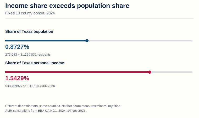
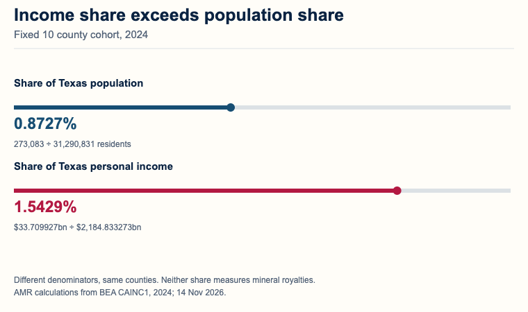
Figure 6 in text
How large is the cohort in Texas? 2024 fixed cohort:0.8727%ofTexas population and1.5429%ofTexas personal income. Shares use different state totals.
Income share exceeds population share Fixed 10 county cohort, 2024
Share of Texas population
0.8727% 273,083 ÷ 31,290,831 residents
Share of Texas personal income
1.5429% $33.709927bn ÷ $2,184.833273bn Different denominators, same counties. Neither share measures mineral royalties. AMR calculations from BEA CAINC1, 2024; 14 Nov 2026.
Additional phone figure text: Two shares of Texas · Same counties, different state denominators. · AMR from BEA CAINC1, 2024; 14 Nov 2026.
Source and data: BEA, CAINC1 state and county totals
Permanent link to this figure’s text and data · Sources and context
What are the exact state share denominators?
Each share uses the matching state total for the same year and measure. The personal income denominator cannot be substituted for the population denominator, even when the resulting percentages are compared in one chart.
The cohort's 273,083 residents divided by Texas's 31,290,831 residents gives 0.8727253%, displayed as 0.8727%. Its $33.709927 billion in personal income divided by Texas's $2,184.833273 billion gives 1.5429062%, displayed as 1.5429%. The counties and year are identical in both calculations. (AMR calculations from BEA, Feb 2026).
In 2010, the group's population share was 0.9035% and its personal income share was 1.3389%. Thus the selected counties gained residents over the full period while their share of Texas population decreased. A falling share does not require a falling headcount when the state population also changes. (AMR calculations from BEA, Feb 2026).
The state shares and the combined income per resident comparison are related, but their labels remain different. A group's income share exceeding its population share is consistent with its combined income per resident exceeding the state's. The source totals make that relationship inspectable.
How were the ten oil counties selected?
The selection is a fixed published production cohort, not an income screen. RRC's April 1, 2024 release provides a preliminary ranking for January 2024 crude oil production, explicitly warning that late and corrected reports can change the production figures.
The ten counties, in that source's production order, are Midland, Martin, Upton, Loving, Howard, Karnes, Reeves, Reagan, Andrews and Glasscock. The source defines crude oil as oil produced from oil leases and excludes condensate, which it reports separately. This article preserves those names for every income year. (Railroad Commission of Texas, Apr 2024).
Midland's preliminary January 2024 oil volume was 16,722,501 barrels, Martin's 16,321,954 and Upton's 7,768,425. The selection download preserves all ten published volumes, their preliminary status and the oil lease scope. These volumes establish the cohort rule; the income analysis does not treat them as final annual production totals. (Railroad Commission of Texas, Apr 2024).
The group is not described as today's ten largest oil producing counties, the ten annual leaders, or the highest income counties in Texas. Each would require a different selection and source. Freezing the cohort avoids replacing members in historical years merely because their production or income position changed.
RRC revision behavior is covered separately in the Texas oil and gas production revisions reference. That issue explains why this page retains the preliminary selection label even though its income values come from a later BEA file.
Does this prove that oil production caused higher resident income or royalties?
The comparison establishes an association between a defined set of oil producing places and their resident income observations. It does not estimate an oil production effect, assign the income to a particular industry, or measure private mineral owner receipts.
CAINC1 has three input measures here: personal income, population and PCPI. None separately identifies mineral royalties, royalty owner counts, ownership fractions or the amount paid to owners living outside the county. Applying a supposed royalty percentage to the income total would create a statistic the source does not contain. (BEA, CAINC1 summary and definitions, Feb 2026).
A causal analysis would need an explicit comparison design and evidence addressing other drivers of income and population. An industry income breakdown, output measure or price series can add context, but none automatically turns this descriptive cohort into a causal experiment.
For publication, preserve four elements beside any selected statistic: the fixed January 2024 preliminary production cohort, the BEA income year, the exact income or population measure, and its denominator. If reporting rank, add that it is among all 254 Texas counties using reported PCPI. If reporting growth, add that the dollars are nominal and the window is 2010 through 2024.
The federal mineral revenue disbursements reference examines public resource money with separate fund definitions. Public mineral disbursements, resident personal income and private royalties are different quantities, and keeping their source systems distinct makes each statistic more useful.
Methodology and sources
AMR fixed ten county names from RRC's preliminary January 2024 oil table before analyzing income. BEA CAINC1 supplies personal income, population and reported PCPI for all 254 Texas counties plus Texas, 2010 through 2024. The pinned file was updated February 5, 2026, with new 2024 statistics and revised 2020 through 2023 values. Ranks use reported PCPI with competition ties. Combined income per resident divides summed income times 1,000 by summed population; unweighted county means and medians treat places equally. Growth uses unrounded quotients. Every essential source cell is populated. No missing value becomes zero, no inflation adjustment or causal attribution is applied, and personal income is not mineral royalty income. This November 14, 2026 analytical edition contains no unreleased 2025 county observations. Downloads preserve all inputs, units, definitions and reproducible calculations. (BEA CAINC1, Feb 2026).
Glossary
- Personal income: income received by or on behalf of an area's residents, following BEA's defined components and adjustments.
- Per capita personal income, PCPI: personal income divided by resident population. It is an area quotient, not median household income.
- Combined cohort quotient: the sum of the selected counties' personal income divided by their combined population, with income converted from thousands of dollars to dollars first.
- Unweighted county median: the middle county PCPI value after ordering the ten county observations; for ten values, the middle two are averaged.
- Unweighted county mean: the sum of the ten published county PCPIs divided by ten, giving each county the same weight.
- Fixed cohort: the same named counties retained in every year, selected by an explicit rule before viewing the income outcomes.
- Competition rank: one plus the number of counties with a strictly higher reported PCPI; tied values share a rank.
- Nominal or current dollars: dollar values without an inflation adjustment. Their growth is not a direct purchasing power measure.
- Population share: cohort residents divided by Texas residents for the same year, expressed as a percentage.
- Preliminary production: an initial reported production observation that the producer may update as late or corrected reports arrive.
Sources
- Bureau of Economic Analysis: CAINC1 county personal income summary, complete CSV archive, definitions and footnotes.
- Bureau of Economic Analysis: Gross Domestic Product by County and Personal Income by County, 2024.
- Bureau of Economic Analysis: Income and Saving learning center.
- Railroad Commission of Texas: Texas Oil and Gas Production Statistics for January 2024, published April 1, 2024.